딥러닝 연습문제 8~15강
8강
#1

i)
import matplotlib.pyplot as plt
import numpy as np

x = np.arange(0,np.pi * 2 , 0.01)


def f(x):
    return np.sin(x)
#g
h = 1e-4
g = (f(x+h) - f(x-h)) / (2*h)


plt.plot(x,f(x))
plt.plot(x,g,color = 'red')
plt.show()
cf) x축을 추가로 그려줘서 명확하게 나타내보자.
+
plt.plot([0,np.pi*2],[0,0], color = 'black')
plt.plot([0,0],[-1,1],color = 'black')
- g(x) 는 f(x)를 미분한것과 같음 즉 cos(x)와 비슷하다라는 걸 알 수 있음.
ii)
- 표준 정규분포를 따라 랜덤하게 1000개의 실수를 뽑는다고 하였으니
- np.random.randn() 함수를 이용해주면 된다.
cf)
- np.random.randn() --> 표준 정규분포를 따라 랜덤하게 추출
- np.random.rand() --> 0~1 까지의 균등분포를 따라 랜덤하게 추출
x = np.random.randn(1000)
- code
import numpy as np

x = np.random.randn(1000)


def f(x):
    return np.sin(x)

def f_prime(x):
    return np.cos(x)
#g
h = 1e-4
g = (f(x+h) - f(x-h)) / (2*h)

result = np.mean(np.abs(f_prime(x)-g))
print(result)
1.1677487977623454e-09
--> 차이는 엄청 미세하다라는 걸 알수있음
Q) 만약 g(x) = f(x+h)-f(x) / h 라면 어떻게 될까 ?
실제로 비교해보자.
import matplotlib.pyplot as plt
import numpy as np

x = np.random.randn(1000)


def f(x):
    return np.sin(x)

def f_prime(x):
    return np.cos(x)
#g
h = 1e-4
g = (f(x+h) - f(x-h)) / (2*h)
g1 = (f(x+h)- f(x)) / h

result_g = np.mean(np.abs(f_prime(x)-g))

result_g1 = np.mean(np.abs(f_prime(x)-g1))

print(result_g)
print(result_g1)
- result
1.1823396151853291e-09
2.825365499384798e-05
- f(x+h) - f(x-h) / 2h 가 f(x+h) - f(x) / h 보다 더욱 더 정밀 하다라는것을 알 수 있음
iii)
import matplotlib.pyplot as plt
import numpy as np

x = np.arange(-10,10,0.01)


def f(x):
    return 1/(1+np.e**(-x))

def f_prime(x):
    return f(x)(1-f(x))
#g
h = 1e-4
g = (f(x+h) - f(x-h)) / (2*h)


plt.plot(x,f(x))
plt.plot(x,g,color = 'red')
plt.plot([-10,10],[0,0], color = 'gray',linestyle = '--')
plt.plot([0,0],[0,1],color = 'gray',linestyle = '--')
plt.show()
import matplotlib.pyplot as plt
import numpy as np

x = np.random.randn(1000)


def f(x):
    return 1/(1+np.e**(-x))

def f_prime(x):
    return f(x)*(1-f(x))
#g
h = 1e-4
g = (f(x+h) - f(x-h)) / (2*h)


result = np.mean(np.abs(f_prime(x)-g))
print(result)
cf) sigmoid' = (sigmoid)(1-sigmoid)
1.238451400598084e-10
#2

import numpy

def f(x):
    return np.sum(x**2)

x = np.ones(3,dtype = float)
# x == [1. , 1., 1.]
grad = np.zeros_like(x)
# grad == [0. , 0. , 0.]

h = 0.1 # h : 엡실론(즉 극한값)

for idx in range(x.size): #x.size = (3,)
    tmp_val = x[idx] # tmp_val : 기존의 x list가 변하지 않게 하기 위함
    x[idx] = float(tmp_val) + h
    print(x) #idx가 0 이라면 x = [1.1 , 1. , 1.]
    fxh1 = f(x) # fxh1 : 좌미분계수

    x[idx] = float(tmp_val) - h
    print(x) #idx 가 0 이라면 x= [0.9, 1., 1.]
    fxh2 = f(x) #fxh2 : 우미분계수

    grad[idx] = (fxh1 - fxh2) / (2*h) # idx = 0 이라면 x0에 대하여 편미분한것을 grad에 대입
    print(grad)
    x[idx] = tmp_val #x[idx]를 다시 원위치로 복귀
result
[1.1 1.  1. ]
[0.9 1.  1. ]
[2. 0. 0.]
[1.  1.1 1. ]
[1.  0.9 1. ]
[2. 2. 0.]
[1.  1.  1.1]
[1.  1.  0.9]
[2. 2. 2.]
cf) f(x) = x0 ^2 + x1^2 + x2^2
#3

i)

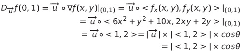
- 점 (0,1)에서 함수 f가 가장 빨리 증가하는 방향은
cos 값이 1인 순간 즉 gradient 방향과 일치할 때 이다. 따라서 <1,2> 이다.
- 점 (0,1)에서 함수 f가 가장 빨리 감소하는 방향은
cos 값이 -1 인 순간 즉 gradient 방향과 반대일 때이다. 따라서 <-1,-2>
- 순간변화율이 0 인 방향은
gradient 방향과 수직일 때이다. 따라서 <-2,1> 또는 <1,-2> 이다.
ii)


- 삼각함수 합성을 이용하여 다음과 같이 sin 에 대한 식으로 변형을 해준다. (실제 손으로 그리기 위해선 다음과 같은 변형은 필수 )

- 파이썬으로 그래프를 그려 확인해보자.
import matplotlib.pyplot as plt
import numpy as np

x = np.arange(0,np.pi * 2 , 0.01)


def f(x):
    return np.sqrt(5) * np.sin(np.arcsin(1/np.sqrt(5)) + x)


plt.plot(x,f(x))
plt.plot([0,np.pi*2],[0,0],color = 'black', linestyle = '--')
plt.show()
- cos a + 2sina 의 그래프도 직접 확인해보면
import matplotlib.pyplot as plt
import numpy as np

x = np.arange(0,np.pi * 2 , 0.01)


def f(x):
    return np.cos(x) + 2 * np.sin(x)


plt.plot(x,f(x))
plt.plot([0,np.pi*2],[0,0],color = 'black', linestyle = '--')
plt.show()
- 동일한 식이라는 것을 확인 가능하다.
iii)
(i) 에서 구한 방향의 편각을 구해보자
- 점 (0,1)에서 함수 f가 가장 빨리 증가하는 방향은
cos 값이 1인 순간 즉 gradient 방향과 일치할 때 이다. 따라서 <1,2> 이다.
--> 편각 : x축과 벡터와의 각도

- 점 (0,1)에서 함수 f가 가장 빨리 감소하는 방향은
cos 값이 -1 인 순간 즉 gradient 방향과 반대일 때이다. 따라서 <-1,-2>
위의 편각에서 + pi 만큼 간거라고 볼 수 있음.

- 순간변화율이 0 인 방향은
gradient 방향과 수직일 때이다. 따라서 <-2,1> 또는 <1,-2> 이다.
기존 arctan2 에서 1/2 pi , 3/2 pi 만큼 더 돌았다라고 의미할수있음.


라는 등식이 만족한다라는 걸 기억해보자.
- 우선 각각의 편각 4개를 ii)의 그래프 위에 나타내보면
import matplotlib.pyplot as plt
import numpy as np

x = np.arange(0,np.pi * 2 , 0.01)


def f(x):
    return np.cos(x) + 2 * np.sin(x)

theta = np.arctan(2)

plt.plot(x,f(x))
plt.plot([0,np.pi*2],[0,0],color = 'black', linestyle = '--')
plt.plot(theta,f(theta),'ro')
plt.plot(theta+np.pi,f(theta+np.pi),'ro')
plt.plot(theta+1/2*np.pi,f(theta+1/2*np.pi),'ro')
plt.plot(theta+3/2*np.pi,f(theta+3/2*np.pi),'ro')


plt.show()
- 다음과 같이 x절편, 극대, 극소에 찍힌다는걸 알 수 있는데
--> 이는 기존 sin를 -arctan2 만큼 평행이동했기 때문이라고 생각하면 좋다.

9강
#1

i)
GD(Gradient Desent)

------------------------------------------------------------------------------------------------


따라서 두걸음 내려갔을 때 위치는 <0 , 3> 이 된다.
ii)
code
# coding: utf-8
import numpy as np
import matplotlib.pylab as plt


def gradient_descent(f, init_x, lr=0.01, step_num=100):
    x = init_x
    x_history = []

    for i in range(step_num):
        x_history.append( x.copy())

        grad = numerical_gradient(f, x)
        x -= lr * grad

    return x, np.array(x_history)


def function(x):
    return x[0]**2 + x[1]**2 + x[0]*x[1] -4*x[0] -8*x[1]

init_x = np.array([0.0, 0.0])

lr = 0.5
step_num = 2
x, x_history = gradient_descent(function, init_x, lr=lr, step_num=step_num)

print(x)
result
[4.66116035e-12 3.00000000e+00]--> 실제로 <0,3> 에 근사한다는것을 알 수 있음
cf) gradient_descent 함수에서 알아가야 할것! --> x_history.append(x.copy())를 해야하는 이유.
def gradient_descent(f, init_x, lr=0.01, step_num=100):
    x = init_x
    x_history = []

    for i in range(step_num):
        x_history.append( x.copy() )

        grad = numerical_gradient(f, x)
        x -= lr * grad

    return x, np.array(x_history)
x_history.append(x.copy())를 해야하는 이유는 x는 리스트의 id 즉 주소값을 받게됨
--> 그래서 x가 변하게 될경우 같이 변하게 됨.
ex)
x = [1,2,3]
y = x

x[0] = 4
print(y)


------

result

[4,2,3]
- 이를 방지하고자 copy() 메소드를 이용해서 직접복사를 해주어 해결할 수 있음
ex)
x = [1,2,3]
y = x.copy()

x[0] = 4
print(y)

---------------
result

[1, 2, 3]
만약에 gradient_descent 함수에서 .copy()메소드가 빠지면 어떻게 될까?
I) copy() O
[[0. 0.]
 [2. 4.]]
II) copy() X
[[4.66116035e-12 3.00000000e+00]
 [4.66116035e-12 3.00000000e+00]]
--> 이렇듯 모든 x의 발자취가 마지막 발자취로 전부 기록이 되게됨
Q) 왜 (2,4) 가 아닌 (0,3) 일까?
- 코드를 보면 x_history에 먼저 append를 하고 그후 x 가 update되는 형식임.
- 따라서 그 x가 update되었기 때문에 그 x값이 모든 발자취를 대체하게 됨.
Q) 기존의 x_history 는 현재의 발자취가 아닌 바로 직전까지의 발자취만 담게된다. 현재 발자취를 담으려면?
def gradient_descent(f, init_x, lr=0.01, step_num=100):
    x = init_x
    x_history = []

    for i in range(step_num):
        x_history.append( x.copy() )

        grad = numerical_gradient(f, x)
        x -= lr * grad

    return x, np.array(x_history)
- 해당 코드에서 x_history.append(x.copy())를 for문 맨 마지막으로 옮겨주면된다. 그리고 for문 바로 직전에 append를 해주면됨
ex)
def gradient_descent(f, init_x, lr=0.01, step_num=100):
    x = init_x
    x_history = []
    x_history.append( x.copy() )
    for i in range(step_num):
        grad = numerical_gradient(f, x)
        x -= lr * grad
        x_history.append( x.copy() )

    return x, np.array(x_history)
result
[[0.00000000e+00 0.00000000e+00]
[2.00000000e+00 4.00000000e+00]
[4.66116035e-12 3.00000000e+00]]
iii)


그러므로 극솟값을 가진다는 것을 알 수 있음.
cf) 이계 도함수 판정법


iv)
# coding: utf-8
import numpy as np
import matplotlib.pylab as plt
from gradient_2d import numerical_gradient


def gradient_descent(f, init_x, lr=0.01, step_num=100):
    x = init_x
    x_history = []
    x_history.append( x.copy() )
    for i in range(step_num):
        grad = numerical_gradient(f, x)
        x -= lr * grad
        x_history.append( x.copy() )

    return x, np.array(x_history)


def function(x):
    return x[0]**2 + x[1]**2 + x[0]*x[1] -4*x[0] -8*x[1]

init_x = np.array([0, 0],dtype = float)

lr = 0.1
step_num = 30
x, x_history = gradient_descent(function, init_x, lr=lr, step_num=step_num)


plt.plot( [-5, 5], [0,0], '--b')
plt.plot( [0,0], [-5, 5], '--b')
plt.plot(x_history[:,0], x_history[:,1], 'ro')

plt.xlim(-1.0, 5.0)
plt.ylim(-1.0, 5.0)
plt.xlabel("X0")
plt.ylabel("X1")
plt.show()

--> 실제로 극솟값인 (0,4)에 근사한다는것을 알 수 있음.
v)
code
# coding: utf-8
import numpy as np
import matplotlib.pylab as plt
from gradient_2d import numerical_gradient


def gradient_descent(f, init_x, lr=0.01, step_num=100):
    x = init_x
    x_history = []
    x_history.append( x.copy() )
    for i in range(step_num):
        grad = numerical_gradient(f, x)
        x -= lr * grad
        x_history.append( x.copy() )

    return x, np.array(x_history)


def function(x):
    return x[0]**2 + x[1]**2 + x[0]*x[1] -4*x[0] -8*x[1]

init_x = np.array([0, 0],dtype = float)

lr = 0.1
step_num = 30
x, x_history = gradient_descent(function, init_x, lr=lr, step_num=step_num)


x = np.arange(-1, 5, 0.1)
y = np.arange(-1, 5, 0.1)
X, Y = np.meshgrid(x, y)

Z=X**2+Y**2 +X*Y -4*X - 8*Y


plt.plot( [-5, 5], [0,0], '--b')
plt.plot( [0,0], [-5, 5], '--b')
plt.plot(x_history[:,0], x_history[:,1], 'ro',markersize = 5)

plt.contour(X,Y,Z,levels = 30) #levels : 등위곡선의 개수를 의미함

plt.xlim(-1.0, 5.0)
plt.ylim(-1.0, 5.0)
plt.xlabel("X0")
plt.ylabel("X1")
plt.show()
--> 등위곡선과 수직인 방향 즉 gradient 방향의 반대방향으로 간다는 것을 알 수 있음.
#2

import numpy as np
import matplotlib.pyplot as plt

def f(x):
    return x*(x-1.0)*(x-2.0)*(x-4.0)

def df(x):
    return (x-1.0)*(x-2.0)*(x-4.0)+x*(x-2.0)*(x-4.0)+x*(x-1.0)*(x-4.0)+x*(x-1.0)*(x-2.0)

lr = 0.02
step = 10

init_position = [0.0, 1.0, 2.0, 4.0]
X = np.arange(-4,5 ,0.01)
Y = f(X)
plt.figure(figsize=(10,10))

for i in range(4):
    x = init_position[i]
    x_history = []
    x_history.append(x)
    for _ in range(step):
        x -= lr * df(x)
        x_history.append(x)

    plt.subplot(2,2,i+1)
    plt.plot(X,Y,color = 'skyblue')
    plt.plot(x_history,f(np.array(x_history)),'ro')
    plt.xlim(-8,8)
    plt.ylim(-8,8)
plt.show()
--> 알아가야하는 것: 시작위치가 매우 중요! (0,1)일땐 최솟값을 향해 가지 않음.
Q1) plt.plot(np.array(x_history), f(np.array(x_history)), 'ro')에서 왜 np.array(x_history)를 하는가?
--> 일반적인 리스트는 f(x_history)를 하게 될 경우 계산이 안되서
--> ndarray 타입으로 변경해줘서 각각의 요소마다 적용이 되게끔 해줘야 한다.
Q2) np.array(history) 를 안쓰고 싶다면 어떻게 해야하나?
- list(map(f,x_history)) --> map 함수를 이용해서 각각의 요소에 대해 적용시켜주면 됨.
10강
#1

i)
1. 수치미분 시간
#수치미분
import sys, os
sys.path.append(os.pardir)  # 부모 디렉터리의 파일을 가져올 수 있도록 설정
import numpy as np
import matplotlib.pyplot as plt
from dataset.mnist import load_mnist
from two_layer_net import TwoLayerNet
from time import time

# 데이터 읽기
(x_train, t_train), (x_test, t_test) = load_mnist(normalize=True, one_hot_label=True)

network = TwoLayerNet(input_size=784, hidden_size=50, output_size=10)

x = x_train[:100]
t = t_train[:100]
lr = 1

#numerical gradient
start = time()
grad = network.numerical_gradient(x, t)
for key in ('W1','b1','W2','b2'):
    network.params[key] -= lr * grad[key]
print('time for numerical_gradient: ',time()-start)

------------------------------------------------------------------------------------
result

time for numerical gradient :  63.685441970825195
2. 역전파 시간
# coding: utf-8
import sys, os
sys.path.append(os.pardir)  # 부모 디렉터리의 파일을 가져올 수 있도록 설정
import numpy as np
import matplotlib.pyplot as plt
from dataset.mnist import load_mnist
from two_layer_net import TwoLayerNet

from time import time

# 데이터 읽기
(x_train, t_train), (x_test, t_test) = load_mnist(normalize=True, one_hot_label=True)

network = TwoLayerNet(input_size=784, hidden_size=50, output_size=10)

x = x_train[:100]
t = t_train[:100]
lr = 1

#backpropagation
start = time()
grad = network.gradient(x, t)
for key in ('W1','b1','W2','b2'):
    network.params[key] -= lr * grad[key]
print('time for backpropagation: ',time()-start)

---------------------------------------------------------------------------
result

time for backpropagation:  0.018896818161010742
- 거의 3000배 가까이 차이난다는 것을 확인 할 수 있다.
ii)
1. 은닉층 뉴런 개수 1개

2. 은닉층 뉴런 개수 2개

3. 은닉층 뉴런 개수 5개

4. 은닉층 뉴런 개수 50개

5. 은닉층 뉴런 개수 200개

cf) 은닉층 뉴런개수에 따른 accuracy를 시각화 해보자.
code : 간단하게 for 문을 이용하여 hidden_size를 변경해주고 최종 정확도를 따로 리스트에 담아서
--> hidden_size의 뉴런개수에 따른 정확도를 대응시켜서 그래프를 그려주면 된다.
# coding: utf-8
import sys, os
sys.path.append(os.pardir)  # 부모 디렉터리의 파일을 가져올 수 있도록 설정
import numpy as np
import matplotlib.pyplot as plt
from dataset.mnist import load_mnist
from two_layer_net import TwoLayerNet

from time import time

# 데이터 읽기
(x_train, t_train), (x_test, t_test) = load_mnist(normalize=True, one_hot_label=True)
test_list = []
for i in range(1,110,10):
    network = TwoLayerNet(input_size=784, hidden_size=i, output_size=10)


    # 하이퍼파라미터
    iters_num = 10000  # 반복 횟수를 적절히 설정한다.
    train_size = x_train.shape[0]
    batch_size = 100   # 미니배치 크기
    learning_rate = 0.1

    train_loss_list = []
    train_acc_list = []
    test_acc_list = []


    # 1에폭당 반복 수
    iter_per_epoch = max(train_size / batch_size, 1)

    for i in range(iters_num):
        # 미니배치 획득
        batch_mask = np.random.choice(train_size, batch_size)
        x_batch = x_train[batch_mask]
        t_batch = t_train[batch_mask]

        # 기울기 계산
        #grad = network.numerical_gradient(x_batch, t_batch)
        grad = network.gradient(x_batch, t_batch)
        # 매개변수 갱신
        for key in ('W1', 'b1', 'W2', 'b2'):
            network.params[key] -= learning_rate * grad[key]


    train_acc = network.accuracy(x_train, t_train)
    test_acc = network.accuracy(x_test, t_test)
    test_list.append(test_acc)

print(test_list)

# 그래프 그리기
x = np.arange(1,110,10)
plt.plot(x, test_list)
plt.xlabel("number of hidden size")
plt.ylabel("accuracy")
plt.xlim(0,110)
plt.ylim(0.94, max(test_list)+0.01)
plt.show()
result
test_list = [0.2853, 0.9198, 0.94, 0.9435, 0.9439, 0.9447, 0.9467, 0.946, 0.9458, 0.9454,0.9455]
- 실제로 그래프를 확인해보면 60부근에서 최댓값을 찍고 점점 감소한다는거슬 육안으로 확인할 수 잇다.
--> 즉 은닉층의 뉴런개수가 많다하더라도 정확성이 좋다라곤 할 수 없다
iii)
result
...
train acc, test acc | 1.0, 0.9707
train acc, test acc | 1.0, 0.9704
train acc, test acc | 1.0, 0.9711
train acc, test acc | 1.0, 0.9709
train acc, test acc | 1.0, 0.9706
train acc, test acc | 1.0, 0.9709
train acc, test acc | 1.0, 0.9707
train acc, test acc | 1.0, 0.971
train acc, test acc | 1.0, 0.9707
train acc, test acc | 1.0, 0.9704
train acc, test acc | 1.0, 0.9704
train acc, test acc | 1.0, 0.9711
train acc, test acc | 1.0, 0.971
- train set의 정확성은 점점 증가하지만
- test set의 정확성은 정체되거나 감소하기도 함
--> 학습횟수가 많다고 해서 신경망의 정확도가 증가한다고 볼 수 없다.
--> 이를 과적합이라고 함.
#2

#!/usr/bin/env python3
# -*- coding: utf-8 -*-
"""
Created on Mon May 27 10:57:24 2024

@author: isuhyeon
"""
import numpy as np
import matplotlib.pyplot as plt


def loss(y,t):
    return np.mean(0.5*(y-t)**2)


x = np.array([[0,0],[0,1],[1,0],[1,1]])
t = np.array([1,0,0,0])

W = np.random.randn(2)
b = 0

for step in range(8):
    threshold = 0.5
    X = np.array([-1,2])
    Y = (threshold-b-W[0]*X)/W[1]

    y = np.sum(x *W,axis = 1) + b

    W[0] -= (2*W[0]+W[1]+2*b-1)/4
    W[1] -= (W[0]+2*W[1]+2*b-1)/4
    b  -= (2*(W[0]+W[1]+2*b)-1)/4

    plt.subplot(2,4,step+1)

    plt.plot([-1,2],Y,color = 'red')
    plt.plot(x[y>0.5][:,0],x[y>0.5][:,1],'bo')
    plt.plot(x[y<=0.5][:,0],x[y<=0.5][:,1],'bx')
    plt.xlim(-1,2)
    plt.ylim(-1,2)

plt.show()
result

- Numerical gradient를 사용하여 Gradient Desent를 해도 되지만
- 나는 정확한 값을 찾기 위해서 실제로 미분을 해봄


- 다음코드가 이를 이용해 Gradient Desent 한다.
    W[0] -= (2*W[0]+W[1]+2*b-1)/4
    W[1] -= (W[0]+2*W[1]+2*b-1)/4
    b  -= (2*(W[0]+W[1]+2*b)-1)/4
12강
#1

i)


ii)
import numpy as np
class Affine:
    def __init__(self, W, b):
        self.W = W
        self.b = b

        self.x = None
        self.original_x_shape = None
        # 가중치와 편향 매개변수의 미분
        self.dW = None
        self.db = None

    def forward(self, x):
        # 텐서 대응
        self.original_x_shape = x.shape
        x = x.reshape(x.shape[0], -1)
        self.x = x

        out = np.dot(self.x, self.W) + self.b

        return out

    def backward(self, dout):
        dx = np.dot(dout, self.W.T)
        self.dW = np.dot(self.x.T, dout)
        self.db = np.sum(dout, axis=0)

        dx = dx.reshape(*self.original_x_shape)  # 입력 데이터 모양 변경(텐서 대응)
        return dx

check = Affine(np.array([[1,2,3],[4,5,6]]),np.array([7,8,9]))
dout = np.array([[2,1,-1],[1,0,0],[0,0,1]])
check.forward(np.array([[1,0],[0,1],[1,1]]))
check.backward(dout)

print(check.db,'\n')
print(check.dW,'\n')
print(check.backward(dout))
result

------------------------------------------------------------

[3 1 0]

[[2 1 0]
 [1 0 1]]

[[1 7]
 [1 4]
 [3 6]]
--> 검산해서 정확히 성립한다는 것을 알 수 있음.
iii)


#2

- 선형변환이므로 다음과 같은 transformation 이 만족함


13강
#1

i)

ii)
import numpy as np
def sigmoid(x):
    return 1 / (1 + np.exp(-x))

class Sigmoid:
    def __init__(self):
        self.out = None

    def forward(self, x):
        out = sigmoid(x)
        self.out = out
        return out

    def backward(self, dout):
        dx = dout * (1.0 - self.out) * self.out

        return dx


x = np.log(np.array([[2,3,4,5],[6,7,8,9]]))

dout = np.array([[3,4,5,6],[7,8,9,10]]) ** 2

S = Sigmoid()

S.forward(x)
S.backward(dout)

print(S.backward(dout))
result
----------------------------------------------------------------

[[2. 3. 4. 5.]
 [6. 7. 8. 9.]]
#2
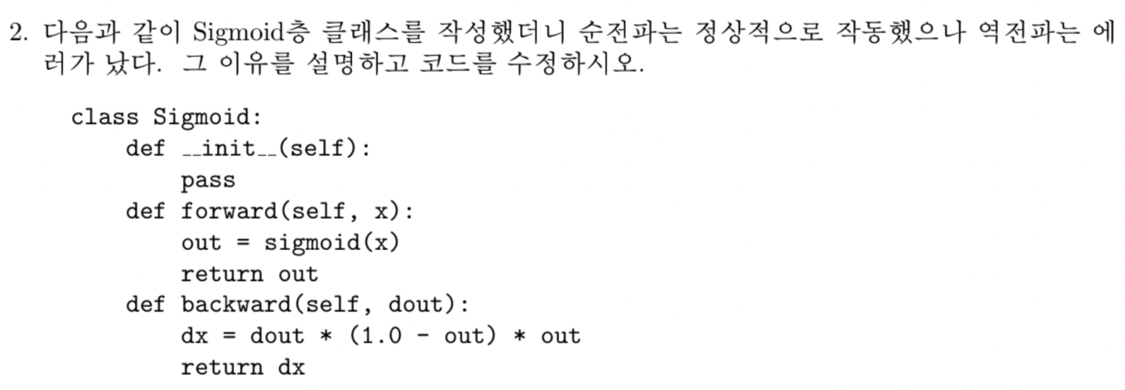
--> out --> self.out 으로 변경해야 함
- backward 메서드 에서는 로컬 변수 out을 인지못한다. 따라서 self.out 으로 글로벌 변수로 만들어줘야함
#3

i)

ii)
import numpy as np
class Relu:
    def __init__(self):
        self.mask = None

    def forward(self, x):
        self.mask = (x <= 0)
        out = x.copy()
        out[self.mask] = 0

        return out

    def backward(self, dout):
        dout[self.mask] = 0
        dx = dout

        return dx

x = np.array([[1,-2,3,-4],[-5,6,-7,8]])
dout = np.array([[1,-2,-3,4],[-1,2,3,-4]])

R = Relu()
R.forward(x)
print(R.backward(dout))
result
[[ 1 0 -3 0]
[ 0 2 0 -4]]
#4

i)
import numpy as np
def sigmoid(x):
    return 1 / (1 + np.exp(-x))

class Relu:
    def __init__(self):
        self.mask = None

    def forward(self, x):
        self.mask = (x <= 0)
        out = x.copy()
        out[self.mask] = 0

        return out

    def backward(self, dout):
        dout[self.mask] = 0
        dx = dout

        return dx

class Sigmoid:
    def __init__(self):
        self.out = None

    def forward(self, x):
        out = sigmoid(x)
        self.out = out
        return out

    def backward(self, dout):
        dx = dout * (10 - self.out) * self.out

        return dx

class Affine:
    def __init__(self, W, b):
        self.W = W
        self.b = b

        self.x = None
        self.original_x_shape = None
        # 가중치와 편향 매개변수의 미분
        self.dW = None
        self.db = None

    def forward(self, x):
        # 텐서 대응
        self.original_x_shape = x.shape
        x = x.reshape(x.shape[0], -1)
        self.x = x

        out = np.dot(self.x, self.W) + self.b

        return out

    def backward(self, dout):
        dx = np.dot(dout, self.W.T)
        self.dW = np.dot(self.x.T, dout)
        self.db = np.sum(dout, axis=0)

        dx = dx.reshape(*self.original_x_shape)  # 입력 데이터 모양 변경(텐서 대응)
        return dx


x = np.random.rand(1,100)
net = []
b = np.zeros(100)
for i in range(10):
    W = 0.01* np.random.randn(100,100)
    net.append(Affine(W,b))
    if i !=9:
        net.append(Sigmoid())


for j in range(19):
    x = net[j].forward(x)

dout = np.random.rand(1,100)

for k in range(len(net)-1,-1,-1):
    dout = net[k].backward(dout)
    if k % 2 ==0:
        print('----')
        print(np.sum((net[k].dW)**2))
        print('----')
result

----
888.3336425782584
----
----
172.99418575762883
----
----
46.213575745705285
----
----
13.545077439041599
----
----
3.0599428733203515
----
----
0.7082805750138639
----
----
0.15764649675159897
----
----
0.02885070372503019
----
----
0.0072572296529022475
----
----
0.002081051011324669
----
ii)
----
2.7511408105771924
----
----
3.093237449986254
----
----
1.8799481050712323
----
----
1.9803168181460404
----
----
1.9000958678427784
----
----
2.230269006710831
----
----
1.59861013624359
----
----
1.6169442592935757
----
----
1.6888406424707738
----
----
1.4737217634288489
----
- sigmoid 층은 0에서 멀어지면 멀어질수록 gradient 가 0 에 수렴하게됨
--> vanishing gradient 현상이 발동됨
--> 이를 해결하기 위해 Relu를 도입하여 해결
14강
#1

1) print(t.size == y.size)
--> t.size = (2, 3) , y.size = (2,3) --> t.size == y.size -> True
2) print(dx)
y : softmax(x) = np.arrray([[0.2,0.3,0.5],[0.7,0.2,0.1]])
t = np.array([[0,0,1],[1,0,0]])
y -t = np.array([[0.2, 0.3, -0.5],[-0.3, 0.2, 0.1]])
--> dx = np.array([[0.2, 0.3, -0.5],[-0.3, 0.2, 0.1]]) / 3 = [[0.2/3, 0.3/3, -0.5/3],[-0.3/3, 0.2/3, 0.1/3]]
3) t = np.argmax(t,axis = 1) ==> [2,0]
print(t) : [2,0]
4) print(t.size:(2,) == y.size:(2,3)) : False
5) print(dx) :
-> dx = np.array([[0.2, 0.3, -0.5],[-0.3, 0.2, 0.1]]) / 3 = [[0.2/3, 0.3/3, -0.5/3],[-0.3/3, 0.2/3, 0.1/3]]
15강
#1

i)
lsh = TwoLayerNet(3, 3, 3)
ii)
x = np.array([[1,2,3],[4,5,6]])
lsh.predict(x)

------------------------------------------------------------------------------------
array([[-0.00016728,  0.00045999, -0.00027152],
       [-0.00031257,  0.0012156 , -0.00063325]])
iii)
t = np.array([[1,0,0],[0,0,1]])

lsh.loss(x,t)

------------------------------------------------------------------------

result

1.0986520249798957
iv)
grad = lsh.gradient(x, t)
print(lsh.params['W1'] - 0.1 * grad['W1'])

---------------------------------------------------------------------------------
result

[[-0.00439563 -0.00577213 -0.00387942]
 [-0.00344992 -0.01167157  0.00203075]
 [ 0.00309354  0.01328105 -0.0080494 ]]
#2


First Print
-

Second Print

#3

i)


------------------------------------------------------------------------------------------


ii)
W1 = np.array([[np.log(2),np.log(2),0],[np.log(2),0,np.log(2)]])
b1 = np.zeros(3)
W2 = np.array([[9,0],[0,5],[0,6]])
b2 = np.zeros(2)

affine1 = Affine(W1,b1)
affine2 = Affine(W2,b2)
sigmoid = Sigmoid()
softmaxwithloss = SoftmaxWithLoss()


x1 = np.array([[2,1]])
t = np.array([[1,0]])

y1 = affine1.forward(x1)
x2 = sigmoid.forward(y1)
y2 = affine2.forward(x2)
loss = softmaxwithloss.forward(y2,t)

dy2 = softmaxwithloss.backward()
dx2 = affine2.backward(dy2)
dy1 = sigmoid.backward(dx2)
dx1 = affine1.backward(dy1)

print("첫번째 Affine층 가중치행렬에 대한 미분 :\n"+str(affine1.dW))
print("첫번째 Affine층 편향벡터에 대한 미분 :\n"+str(affine1.db))
print("두번째 Affine층 가중치행렬에 대한 미분 :\n"+str(affine2.dW))
print("두번째 Affine층 편향벡터에 대한 미분 :\n"+str(affine2.db))

--------------------------------------------------------------------------------------------
result

첫번째 Affine층 가중치행렬에 대한 미분 :
[[-0.88888889  0.8         1.33333333]
 [-0.44444444  0.4         0.66666667]]

첫번째 Affine층 편향벡터에 대한 미분 :
[-0.44444444  0.4         0.66666667]

두번째 Affine층 가중치행렬에 대한 미분 :
[[-0.44444444  0.44444444]
 [-0.4         0.4       ]
 [-0.33333333  0.33333333]]

두번째 Affine층 편향벡터에 대한 미분 :
[-0.5  0.5]
iii)
print(W1 - affine1.dW)
print(b1 - affine1.db)
print(W2 - affine2.dW)
print(b2 - affine2.db)

----------------------------------------------------------------------------------
result

W1
[[ 1.58203607 -0.10685282 -1.33333333]
 [ 1.13759163 -0.4         0.02648051]]

b1
[ 0.44444444 -0.4        -0.66666667]

W2
[[ 9.44444444 -0.44444444]
 [ 0.4         4.6       ]
[ 0.33333333  5.66666667]]

b2
[ 0.5 -0.5]
#4

i)


ii)
W1 = np.array([[0,0,0,0,1],[1,0,0,0,0],[0,-1,0,0,0],[0,0,-1,0,0],[0,0,0,-1,0]])
b1 = np.zeros(5)
W2 = np.array([[5,0,0,0,5],[5,0,0,0,5],[5,0,0,0,5],[5,0,0,0,5],[-5,5,5,5,-5]])
b2 = np.zeros(5)

affine1 = Affine(W1,b1)
affine2 = Affine(W2,b2)
relu = Relu()
softmaxwithloss = SoftmaxWithLoss()

x1 = np.array([[1,2,3,4,5]])
t = np.array([[1,0,0,0,0]])

y1 = affine1.forward(x1)
x2 = relu.forward(y1)
y2 = affine2.forward(x2)
loss = softmaxwithloss.forward(y2,t)

dy2 = softmaxwithloss.backward()
dx2 = affine2.backward(dy2)
dy1 = relu.backward(dx2)
dx1 = affine1.backward(dy1)

print("첫번째 Affine층 가중치행렬에 대한 미분 :\n"+str(affine1.dW))
print("="*40)
print("첫번째 Affine층 편향벡터에 대한 미분 :\n"+str(affine1.db))
print("="*40)
print("두번째 Affine층 가중치행렬에 대한 미분 :\n"+str(affine2.dW))
print("="*40)
print("두번째 Affine층 편향벡터에 대한 미분 :\n"+str(affine2.db))

------------------------------------------------------------------------
result

첫번째 Affine층 가중치행렬에 대한 미분 :
[[ -3.   0.   0.   0.   6.]
 [ -6.   0.   0.   0.  12.]
 [ -9.   0.   0.   0.  18.]
 [-12.   0.   0.   0.  24.]
 [-15.   0.   0.   0.  30.]]
========================================
첫번째 Affine층 편향벡터에 대한 미분 :
[-3.  0.  0.  0.  6.]
========================================
두번째 Affine층 가중치행렬에 대한 미분 :
[[-1.6  0.4  0.4  0.4  0.4]
 [ 0.   0.   0.   0.   0. ]
 [ 0.   0.   0.   0.   0. ]
 [ 0.   0.   0.   0.   0. ]
 [-0.8  0.2  0.2  0.2  0.2]]
========================================
두번째 Affine층 편향벡터에 대한 미분 :
[-0.8  0.2  0.2  0.2  0.2]
iii)
print(W1-affine1.dW)
print(b1-affine1.db)
print(W2-affine2.dW)
print(b2-affine2.db)


------------------------------------------------------------------------

result

W1
[[  3.   0.   0.   0.  -5.]
 [  7.   0.   0.   0. -12.]
 [  9.  -1.   0.   0. -18.]
 [ 12.   0.  -1.   0. -24.]
 [ 15.   0.   0.  -1. -30.]]

 b1
[ 3.  0.  0.  0. -6.]

W2
[[ 6.6 -0.4 -0.4 -0.4  4.6]
 [ 5.   0.   0.   0.   5. ]
 [ 5.   0.   0.   0.   5. ]
 [ 5.   0.   0.   0.   5. ]
 [-4.2  4.8  4.8  4.8 -5.2]]

b2
[ 0.8 -0.2 -0.2 -0.2 -0.2]
#5

i) 표준편차 : 1
0.13158333333333333 0.1328
0.7812166666666667 0.7903
0.8208833333333333 0.8278
0.844 0.8486
0.8547 0.8585
0.86495 0.8686
0.873 0.8776
0.8743833333333333 0.8723
0.8900666666666667 0.8913
0.8861 0.8881
0.8913666666666666 0.8931
0.89465 0.8979
0.8919666666666667 0.8922
0.8998833333333334 0.9013
0.9061666666666667 0.9082
0.9105166666666666 0.9109
0.91005 0.9124
ii) 표준편차 : 10
0.17435 0.1691
0.7473 0.7579
0.7241666666666666 0.7249
0.6831333333333334 0.6882
0.6262833333333333 0.624
0.592 0.5925
0.5781833333333334 0.5795
0.5706666666666667 0.5774
0.5295833333333333 0.534
0.5638833333333333 0.5575
0.5395 0.5451
0.5460833333333334 0.5411
0.5325166666666666 0.5232
0.49248333333333333 0.4928
0.5407833333333333 0.5382
0.5470333333333334 0.5359
0.5178666666666667 0.5034
--> 표준편차가 증가하니 표준편차가 1일때에 비해 정확도가 뚜렷하게 감소함
iii) 표준편차 : 0
0.10441666666666667 0.1028
0.11236666666666667 0.1135
0.11236666666666667 0.1135
0.11236666666666667 0.1135
0.11236666666666667 0.1135
0.11236666666666667 0.1135
0.11236666666666667 0.1135
0.11236666666666667 0.1135
0.11236666666666667 0.1135
0.11236666666666667 0.1135
0.11236666666666667 0.1135
0.11236666666666667 0.1135
0.11236666666666667 0.1135
0.11236666666666667 0.1135
0.11236666666666667 0.1135
0.11236666666666667 0.1135
0.11236666666666667 0.1135
--> 표준편차를 잡는 것도 굉장히 중요한 일이라는 것을 알 수 있다.
#6


i)
import pickle


with open('fashion_mnist.pkl','rb') as f:
    fashion_mnist = pickle.load(f)

print(fashion_mnist)
--> pkl : Python Dictionary
ii)
print(fashion_mnist.keys())

------------------------------------
result

dict_keys(['x_train', 't_train', 'x_test', 't_test'])
for i in fashion_mnist.values():
    print(i.shape)

---------------------------------------------------------------------------

(60000, 28, 28)
(60000,)
(10000, 28, 28)
(10000,)
iii)
np.set_printoptions(linewidth=200,threshold=1000)

x_train = fashion_mnist['x_train']
t_train = fashion_mnist['t_train']
x_test = fashion_mnist['x_test']
t_test = fashion_mnist['t_test']

print(x_train[0])
- result

iv)
plt.figure(figsize = (10,10))

label = ['T-shirt','Trouser','Pullover',
         'Dress','Coat','Sandal','shirt',
         'Sneaker','Bag','Ankle boot']
for i in range(25):
    plt.subplot(5,5,i+1)
    plt.xticks([])
    plt.yticks([])
    plt.imshow(x_train[i],cmap = plt.cm.binary)
    plt.xlabel(label[t_train[i]])
plt.show()
result

v)
x_train = np.array(fashion_mnist['x_train'],dtype = float)
t_train = fashion_mnist['t_train']
x_test = np.array(fashion_mnist['x_test'],dtype = float)
t_test = fashion_mnist['t_test']


x_train /= 255
x_test /= 255
vi)
# coding: utf-8
import sys, os
sys.path.append(os.pardir)  # 부모 디렉터리의 파일을 가져올 수 있도록 설정
import numpy as np
import matplotlib.pyplot as plt
from dataset.mnist import load_mnist
from two_layer_net import TwoLayerNet
import pickle


with open('fashion_mnist.pkl','rb') as f:
    fashion_mnist = pickle.load(f)

np.set_printoptions(linewidth=200,threshold=1000)

x_train = np.array(fashion_mnist['x_train'],dtype = float)
t_train = fashion_mnist['t_train']
x_test = np.array(fashion_mnist['x_test'],dtype = float)
t_test = fashion_mnist['t_test']


x_train /= 255
x_test /= 255

network = TwoLayerNet(input_size=784, hidden_size=50, output_size=10)

# 하이퍼파라미터
iters_num = 10000  # 반복 횟수를 적절히 설정한다.
train_size = x_train.shape[0]
batch_size = 100   # 미니배치 크기
learning_rate = 0.1

train_loss_list = []
train_acc_list = []
test_acc_list = []

# 1에폭당 반복 수
iter_per_epoch = max(train_size / batch_size, 1)

for i in range(iters_num):
    # 미니배치 획득
    batch_mask = np.random.choice(train_size, batch_size)
    x_batch = x_train[batch_mask]
    t_batch = t_train[batch_mask]

    # 기울기 계산
    #grad = network.numerical_gradient(x_batch, t_batch)
    grad = network.gradient(x_batch, t_batch)

    # 매개변수 갱신
    for key in ('W1', 'b1', 'W2', 'b2'):
        network.params[key] -= learning_rate * grad[key]

    # 학습 경과 기록
    loss = network.loss(x_batch, t_batch)
    train_loss_list.append(loss)

    # 1에폭당 정확도 계산
    if i % iter_per_epoch == 0:
        train_acc = network.accuracy(x_train, t_train)
        test_acc = network.accuracy(x_test, t_test)
        train_acc_list.append(train_acc)
        test_acc_list.append(test_acc)
        print("train acc, test acc | " + str(train_acc) + ", " + str(test_acc))
result
train acc, test acc | 0.1459, 0.1478
train acc, test acc | 0.80945, 0.7996
train acc, test acc | 0.8314666666666667, 0.8183
train acc, test acc | 0.8542666666666666, 0.8398
train acc, test acc | 0.85415, 0.8364
train acc, test acc | 0.8675166666666667, 0.8504
train acc, test acc | 0.87195, 0.8557
train acc, test acc | 0.8712333333333333, 0.8542
train acc, test acc | 0.8771166666666667, 0.8586
train acc, test acc | 0.8831166666666667, 0.8675
train acc, test acc | 0.8821333333333333, 0.8623
train acc, test acc | 0.87475, 0.8522
train acc, test acc | 0.8874, 0.8648
train acc, test acc | 0.8877333333333334, 0.8647
train acc, test acc | 0.8935333333333333, 0.8714
train acc, test acc | 0.8837833333333334, 0.8611
train acc, test acc | 0.8925833333333333, 0.8662
vii)
confusion = np.zeros((10,10),dtype = int)

for k in range(len(x_test)):
    i = t_test[k]
    y = network.predict(x_test[k].reshape(1,784))
    j = np.argmax(y)
    confusion[i,j] +=1

print(confusion)

------------------------------------

[[846   0  14  26   1   1 104   0   8   0]
 [  5 964   1  24   2   0   3   0   1   0]
 [ 17   1 856  12  33   0  80   0   1   0]
 [ 31   6  10 893  19   0  38   0   3   0]
 [  1   1 220  62 579   1 131   0   5   0]
 [  0   0   0   1   0 949   0  29   2  19]
 [145   1 108  27  25   2 680   0  12   0]
 [  0   0   0   0   0  25   0 923   1  51]
 [  8   0  10   4   2   2   9   7 958   0]
 [  1   0   0   0   0   8   0  24   0 967]]
viii)
precision = np.diag(confusion)/ np.sum(confusion, axis = 0)

recall = np.diag(confusion) / np.sum(confusion , axis = 1)

F1_score = 0.5*(1/precision + 1/recall)

------------------------------------------------------------------------

 array([0.82114625, 0.99070248, 0.79118573, 0.80935569, 0.75292004,
 0.94471866, 0.75337423, 0.93460765, 0.96385542, 0.94915254])

 array([0.831, 0.959, 0.754, 0.917, 0.838, 0.957, 0.614, 0.929, 0.96 , 0.952])

 array([1.21058965, 1.02606882, 1.29509284, 1.16303162, 1.26073986,
 1.05172414, 1.47801303, 1.07319699, 1.03958333, 1.0519958 ])
#7


i)
import pickle

with open("cifar10.pkl",'rb') as f:
    cifar10 = pickle.load(f)

print(cifar10)
ii)
print(cifar10.keys())

--------------------------------------------------------------------------------
result

dict_keys(['x_train', 't_train', 'x_test', 't_test'])
for i in cifar10.values():
    print(i.shape)

------------------------------------------------------------------------
x_train
(50000, 32, 32, 3)

t_train
(50000,)

x_test
(10000, 32, 32, 3)

t_test
(10000,)
iii)
l = ['airplane','automobile','bird','cat','deer',
     'dog','frog','horse','ship','truck']

plt.figure(figsize=(10,10))
for i in range(25):
    plt.subplot(5,5,i+1)
    plt.xticks([])
    plt.yticks([])
    plt.imshow(x_train[i], cmap=plt.cm.binary)
    plt.xlabel(l[t_train[i]])
plt.show()
iv)
x_train = np.array(cifar10['x_train'],dtype = float)
t_train = cifar10['t_train']
x_test = np.array(cifar10['x_test'],dtype = float)
t_test = cifar10['t_test']


x_train /= 255
x_test /= 255
v)
# coding: utf-8
import sys, os
sys.path.append(os.pardir)  # 부모 디렉터리의 파일을 가져올 수 있도록 설정
import numpy as np
import matplotlib.pyplot as plt
from dataset.mnist import load_mnist
from two_layer_net import TwoLayerNet

# 데이터 읽기

network = TwoLayerNet(input_size=32*32*3, hidden_size=50, output_size=10)

import pickle

with open("cifar10.pkl",'rb') as f:
    cifar10 = pickle.load(f)


x_train = np.array(cifar10['x_train'],dtype = float)
t_train = cifar10['t_train']
x_test = np.array(cifar10['x_test'],dtype = float)
t_test = cifar10['t_test']


x_train /= 255
x_test /= 255

# 하이퍼파라미터
iters_num = 10000  # 반복 횟수를 적절히 설정한다.
train_size = x_train.shape[0]
batch_size = 100   # 미니배치 크기
learning_rate = 0.1

train_loss_list = []
train_acc_list = []
test_acc_list = []

# 1에폭당 반복 수
iter_per_epoch = max(train_size / batch_size, 1)

for i in range(iters_num):
    # 미니배치 획득
    batch_mask = np.random.choice(train_size, batch_size)
    x_batch = x_train[batch_mask]
    t_batch = t_train[batch_mask]

    # 기울기 계산
    #grad = network.numerical_gradient(x_batch, t_batch)
    grad = network.gradient(x_batch, t_batch)

    # 매개변수 갱신
    for key in ('W1', 'b1', 'W2', 'b2'):
        network.params[key] -= learning_rate * grad[key]

    # 학습 경과 기록
    loss = network.loss(x_batch, t_batch)
    train_loss_list.append(loss)

    # 1에폭당 정확도 계산
    if i % iter_per_epoch == 0:
        train_acc = network.accuracy(x_train, t_train)
        test_acc = network.accuracy(x_test, t_test)
        train_acc_list.append(train_acc)
        test_acc_list.append(test_acc)
        print("train acc, test acc | " + str(train_acc) + ", " + str(test_acc))
train acc, test acc | 0.10008, 0.1008
train acc, test acc | 0.33596, 0.3351
train acc, test acc | 0.38308, 0.3854
train acc, test acc | 0.38484, 0.3814
train acc, test acc | 0.40654, 0.4028
train acc, test acc | 0.4186, 0.4079
train acc, test acc | 0.43124, 0.4204
train acc, test acc | 0.4589, 0.4469
train acc, test acc | 0.39682, 0.3897
train acc, test acc | 0.46108, 0.4496
train acc, test acc | 0.47, 0.4576
train acc, test acc | 0.48382, 0.4604
train acc, test acc | 0.49148, 0.4676
train acc, test acc | 0.48064, 0.4534
train acc, test acc | 0.48748, 0.4538
train acc, test acc | 0.4731, 0.4514
train acc, test acc | 0.5014, 0.4675
train acc, test acc | 0.49374, 0.4649
train acc, test acc | 0.4802, 0.4524
train acc, test acc | 0.49692, 0.4663
#8

i)
x=np.zeros((10000,1,28,28))
    x[:,:,:28-k,k:] = x_test[:,:,k:,:28-k]
ii)
==========평행이동시킨 픽셀 : 1==========
0.9139
==========평행이동시킨 픽셀 : 2==========
0.6206
==========평행이동시킨 픽셀 : 3==========
0.2494
--> 인간은 평행이동, 확대, 축소, 회전한 이미지등은 전부 동일한 이미지라고 인식하지만
--> 딥러닝에서는 flatten한데이터를 바탕으로 학습이 되기 때문에 다른 이미지라고 생각을하게됨.
$$ x=\frac{-b+\sqrt{b^{2}-4ac}}{2a} $$